Basic general question about controllers

Question

Suppose I have a mechanical system which is free to move on a given rail [-5m, 5m] like a motorized cart. The whole system can be mathematically expressed through a linear timeinvariant system equations.

If I need to control only the position (for example saying the controller: "move to +2.3") I can simply design a PID controller that, given a set point moves the cart to that position.

Now I need much more and I want to control the position and the velocity of the cart. So I need for example to say: "move to +2.3 with a specific velocity's profile". Of course the vel = 0 at the end position.

Question: how should I design such a controller? Do I need specifically a special type of controller? Or I have a huge choice?

Any help, graph, link and example is really appreciated.

Regards

Answer 1

PID would work just fine. Your system can be easily modeled as a linear system and is relatively easy to control. When you want to choose a control method, you need to know the dynamics of your system, computation resources, and how much you wanna go deep into mathematical stuff(one reason why so many people choose PID).

To solve your control problem using PID, you need to define your X and Y as functions of time based on your desired velocity. So you will have: $$ X(t), Y(t)$$

Or in case of moving on a rail, define travel distance as a function of time. Then in each iteration of your control loop you know where the cart was supposed to be and where it really is. The difference is the error that you should put in PID equation. It might not always be so straight forward. In most of multi-output control systems error is a mix of multiple state errors(such as path tracking in 2D with differential wheel robots).

The Matlab code below might help you better understand the process. In case you don't have access to Matlab, Octave should be able to run the code too(maybe with some small adjustments).

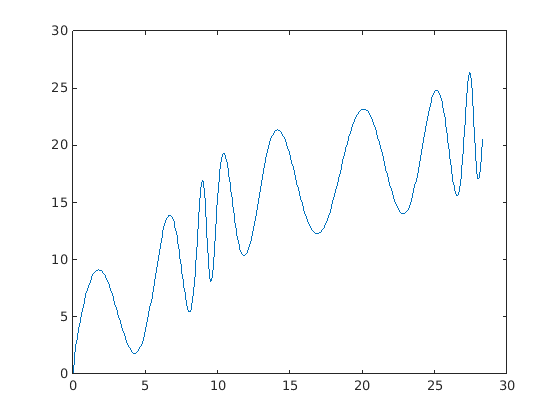
I've assumed that there is a rail that looks like this:

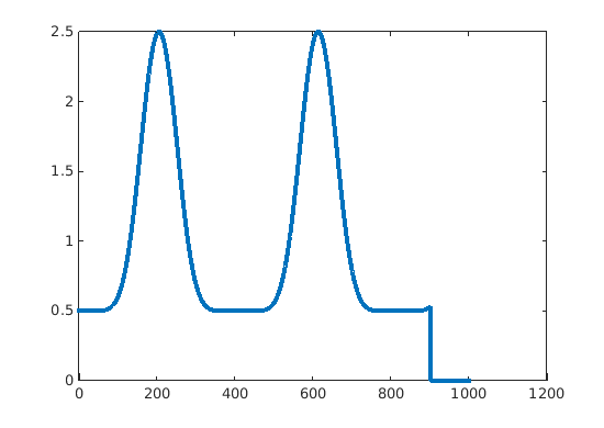
And you want to move on it with a velocity profile like this:

Then follow this example:

clc; clear all; close all

%% Path setup
path_step = transpose(0:.01:500);
x_path = path_step/17 + 2*sin(path_step/50);
y_path = sqrt(path_step) + 5*sin(path_step/10);

position_matrix = [x_path,y_path];
distance_between_points = diff(position_matrix,1);
dist_from_vertex_to_vertex = hypot(distance_between_points(:,1), distance_between_points(:,2));
cumulative_dist_along_path = [0; cumsum(dist_from_vertex_to_vertex,1)];


%% Cart setup
saturation_limit = 4;
motor_coef = .5;
motor_model = @(input_command) min(saturation_limit, max(-saturation_limit, input_command * motor_coef)) + .3 * randn(1);
k_p = 3;
k_i = 1;
k_d = .1;


%% Simulation and initial conditions setup and array initialization
time_step = .1;
sim_time = 100;
t = transpose(0:time_step:sim_time);
distance_actual = zeros(size(t));
err = zeros(size(t));

err_integrated = 0;
err_derivative = 0;
distance_actual(1) = 20; % actual starting point


%% Desired trajectory following pattern
velocity = .5 + 2*sin(t/13).^8;
velocity=[velocity(1:end-100); zeros(100,1)];
reference_starting_point = 40;
desired_travel_distances = cumsum(velocity .* time_step,1) + reference_starting_point; 
desired_trajectory = interp1(cumulative_dist_along_path, position_matrix, desired_travel_distances);
x_pos = desired_trajectory(:,1);
y_pos = desired_trajectory(:,2);

%% Run simulation
for sim_step = 1:sim_time/time_step
    err(sim_step) = desired_travel_distances(sim_step) - distance_actual(sim_step); % calculate error
    err_integrated = err_integrated + err(sim_step) * time_step;
    if sim_step>1
        err_derivative = (err(sim_step) - err(sim_step-1)) / time_step;
    end
    u_motor = k_p * err(sim_step) + k_d * err_derivative + k_i * err_integrated; % apply PID magic and calculate control input
    actual_velocity(sim_step) = motor_model(u_motor); % Send the command to the motor and it will have a new velocity based on that
    distance_actual(sim_step+1) = actual_velocity(sim_step) * time_step + distance_actual(sim_step); % calculate traveled distance from new
end


%% How good it follows the desired velocity pattern
figure()
title('Velocity Profile')
xlabel('Simulation Step')
ylabel('Velocity')
plot(velocity,'LineWidth',3)
hold on
plot(actual_velocity, ':')
hold off
legend('Desired', 'Actual')


%% Error analysis
figure()
title('Error')
xlabel('Simulation Step')
ylabel('Error')
plot(err)


%% Make an animation
actual_position = interp1(cumulative_dist_along_path, position_matrix, distance_actual);
figure()
title('Simulation')
xlabel('X')
ylabel('Y')
plot(x_path, y_path)
hold on
h1 = plot(x_pos(1), y_pos(1), 'rx');
h2 = plot(actual_position(1, 1), actual_position(1, 2), 'ko');
legend('Path', 'Desired Position', 'Actual Position')
disp('Press key ...')
waitforbuttonpress()
for sim_step=1:sim_time/time_step
    delete(h1)
    delete(h2)
    clc
    disp('Time:')
    t = sprintf('%0.3f', sim_step * time_step);
    disp(t)
    h1 = plot(x_pos(sim_step), y_pos(sim_step), 'rx');
    h2 = plot(actual_position(sim_step, 1), actual_position(sim_step, 2), 'ko');
    drawnow
    pause(.05)
end
clc
disp('Finished!')

Answer 2

The best control you can design is "exact feed forward linearization based on differential flatness". This is a complete approach to design control laws for flat systems.

Just PID is not a good idea : you will get overshoot and you do not master precisely position/velocity.

Flatness is a generalization on controllability. Hence you are sure that your system can achieve any position/velocity profile provided you remain inside the physical constraints.