How to solve this differential equation using ode23?

Question

Hello! :) What I have here is a gear system I need to simulate using MATLAB and Simulink.

To do that, firstly I need to get the differential equation for this rotation (gear) system. I think I managed to do so and it is as follows iT1 = J * theta2''+D * theta2'+K * theta2

, where J = i^2 * Jn1 + Jn2 + J2 (also, i is the gear ratio; i = theta1/theta2 = N2/N1 = Tn2 / Tn1 = T2/T1).

Now I need to solve this second-order differential equation using ode23 in MATLAB. The problem is, I don't know any initial conditions, nor do I know how to get them from this particular system e.g. y(0) = 0, y'(0) = 1 Can I still solve this particular problem without the initial conditions, or do I make the initial conditions up...? In case anyone needs it the parameters of my problem are as follows:

N2 = 90, N1 = 36, Jn1 = 0.5 Nms^2/rad, Jn2 = 0.8 Nms^2/rad, J2 = 2 Nms^2/rad, D = 8 Nms/rad, K = 5 Nm/rad

The differential equation should look like this for y=theta2 and x=T1

y''+1.3502y'+0.8439y = 0.4219x

Any help would be really appreciated! :)

Answer 1

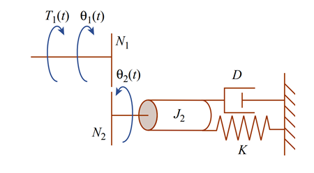
You can certainly employ ode23 to solve this ordinary differential equation, but it's much simpler if you recruit the state space approach via ss and then lsim.

The response of a linear system is always the aggregate of its forced (with a null initial state) and unforced evolutions (with $T_1=0$ and a given initial state $\mathbf{x}_0$).

The unforced evolution can be determined by means of initial.

So, to answer your direct question, the initial conditions (read the initial state) are crucial as they establish part of the transient response of the system.

% parameters
N2  = 90;
N1  = 36;
Jn1 = 0.5;
Jn2 = 0.8;
J2  = 2;
D   = 8;
K   = 5;
J   = (N2/N1)^2 * Jn1 + Jn2 + J2;

% define the system
sys = ss([0 1; -K/J -D/J], [0; N2/(N1*J)], [1 0], 0);

% initial state: (position, velocity) [rad; rad/s]
x0 = [0.1; 0];

% define the time span
t = linspace(0, 15, 10000)';

% define the input step
T1 = zeros(length(t), 1);
T1(t>=1) = 1;

% compute the system step response at once
theta1 = lsim(sys, T1, t, x0);

% compute the system response as aggregate of the forced and unforced
% temporal evolutions
theta2 = lsim(sys, T1, t, [0; 0]) + initial(sys, x0, t);

% plot results
figure('color', 'white');
hold on;
yyaxis left;
plot(t, T1, '-.', 'linewidth', 2);
ylabel('[N]');
yyaxis right;
plot(t, theta1, 'linewidth', 3);
plot(t, theta2, 'k--');
xlabel('t [s]');
ylabel('[rad]');
grid minor;
legend({'$T_1$', '$\theta_1$', '$\theta_2$'}, 'Interpreter', 'latex',...
       'location', 'southeast');
hold off;

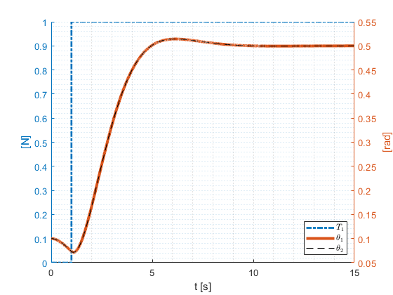
Here's the resulting plot:

---

If you really want to use ode23, then you can run the following snippet:

% initial state: (position, velocity) [rad; rad/s]
x0 = [0.1; 0];

% define the time span
t = linspace(0, 15, 10000)';

% integrate the differential equation
[t, x] = ode23(@fun, t, x0);

% plot results
figure('color', 'white');
plot(t, x(:, 1));
xlabel('t [s]');
ylabel('[rad]');
grid minor;
legend({'$\theta$'}, 'Interpreter', 'latex', 'location', 'southeast');


function g = fun(t, x)
% parameters
N2  = 90;
N1  = 36;
Jn1 = 0.5;
Jn2 = 0.8;
J2  = 2;
D   = 8;
K   = 5;
J   = (N2/N1)^2 * Jn1 + Jn2 + J2;

% compute gradient
g = zeros(2, 1);
g(1) = x(2);
g(2) = (-K/J)*x(1) + (-D/J)*x(2) + (N2/(N1*J)*(t>=1));
end

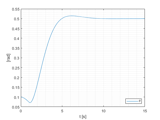
yielding the graph below:

---

Finally, if you aim to integrate a generic input as a function of time $t$, you could resort to the code below:

function x = integrate(t, u, x0)
    % parameters
    N2  = 90;
    N1  = 36;
    Jn1 = 0.5;
    Jn2 = 0.8;
    J2  = 2;
    D   = 8;
    K   = 5;
    J   = (N2/N1)^2 * Jn1 + Jn2 + J2;

    % integrate the differential equation
    [t, x] = ode23(@fun, t, x0);

    % plot results
    figure('color', 'white');
    
    % plot position
    yyaxis left;
    plot(t, x(:, 1));
    ylabel('$x$ [rad]', 'Interpreter', 'latex');
    
    % plot velocity
    yyaxis right;
    plot(t, x(:, 2));
    ylabel('$\dot{x}$ [rad/s]', 'Interpreter', 'latex');
    
    grid minor;
    xlabel('$t$ [s]', 'Interpreter', 'latex');

    function g = fun(t, x)
        g = zeros(2, 1);
        g(1) = x(2);
        g(2) = (-K/J)*x(1) + (-D/J)*x(2) + (N2/(N1*J)*u(t));
    end
end

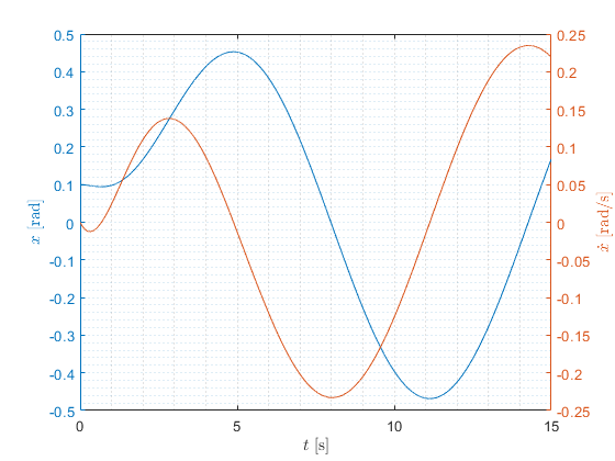
You can now employ anonymous functions to specify the temporal evolution of the input. For example, if the input is sinusoidal with pulse frequency $\omega = 0.5 \; \text{rad/s}$, you'll need to run:

t = linspace(0, 15, 10000)';
x0 = [0.1; 0];
integrate(t, @(t)(sin(0.5*t)), x0);

to get: