I'm going to give you a high-level overview without going into much math. The purpose here is to give you a somewhat intuitive understanding of what is going on, and hopefully this will help the more mathematical resources make more sense. I'm mostly going to focus on the unscented transform, and how it relates to the UKF.
Random variables
Alright, the first thing you need to understand is that modern (mobile) robotics is probabilistic; that is, we represent things we aren't sure about by random variables. I've written about this topic on my personal website, and I strongly suggest you check it out for a review. I'm going to briefly go over it here.
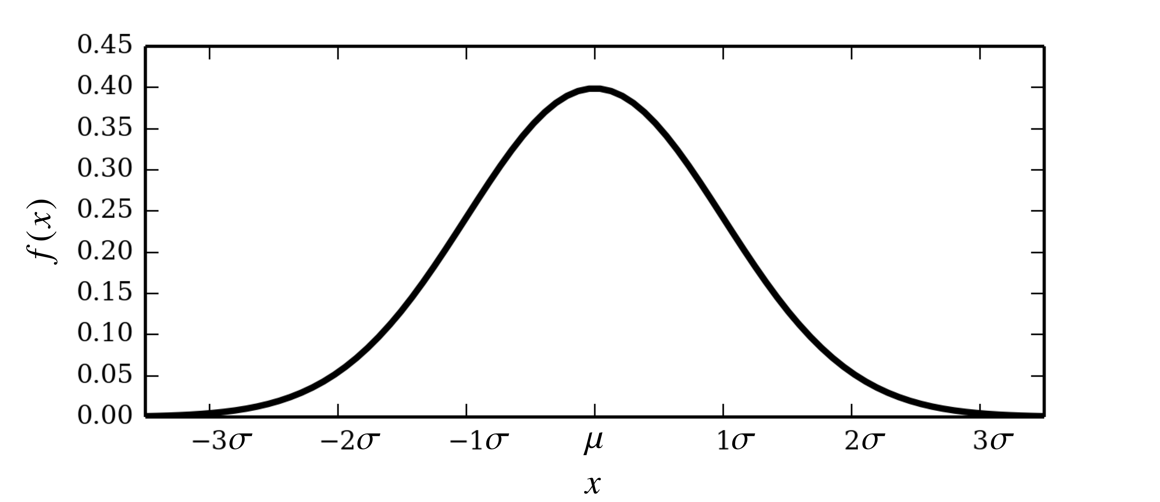
Take the (one-dimensional) position of a robot for example. Usually we use sensors (e.g., wheel encoders, laser scanners, GPS, etc.) to estimate the position, but all of these sensors are noisy. In other words, if our GPS tells us we are at $x = 10.2$ m, there is some uncertainty associated with that measurement. The most common way we model this uncertainty is using Gaussian (also known as Normal) distributions. The probabilistic density function (don't worry about what this means for now) of a Gaussian distribution looks like this:

On the $x$ axis are different values for your random variable. For example, this could be the one dimensional position of the robot. The mean position is denoted by $\mu$, and the standard deviation is denoted by $\sigma$, which is a sort of "plus/minus" applied to the mean. So instead of saying "the robot's position is $x = 9.84$ m", we say something along the lines of "the mean of our estimate of the robot's position is $x = 9.84$ m with a standard deviation of $0.35$ m".
On the $y$ axis is the relative likelihood of that value occurring. For example, note that $x = \mu$ has a relative likelihood of about $0.4$, and $x = \mu - 2\sigma$ has a relative likelihood of about $0.05$. And let's pretend that $\mu = 9.84$ m and $\sigma = 0.35$ m like the above example. That means
$$
\mu = 9.84 \text{ m}, \quad \mu - 2\sigma = 9.84 - 2(0.35) = 9.14 \text{ m}
$$
What the $y$-axis values are telling you is that the likelihood that the robot is at $9.84$ is eight times higher than $9.14$ because the ratio of their likelihoods is $0.4/0.05 = 8$.
The takeaway point from this section is that the things we often most interested in (e.g., position, velocity, orientation) are random variables, most often represented by Gaussian distributions.
Passing random variables through functions
An interesting property of Gaussian random variables is that the result of passing one through a linear function results in a Gaussian random variable. So if we have a function like
$$
y = 12x - 7
$$
and $x$ is a Gaussian random variable, then $y$ is also a Gaussian random variable (but with a different mean and standard deviation). On the other hand, this property does not hold for nonlinear functions, such as
$$
y = 3\sin(x) - 2x^2.
$$
Here, passing the Gaussian random variable $x$ through the function results in a non-Gaussian distribution $y$. In other words, the shape of the PDF for $y$ would not look like the above plot. But what do I mean by "passing a Gaussian random variable through a function". In other words, what do I put in for $x$ in the above equation? As we saw in the above plot, $x$ has many possible values.
As before, let's say $x$ has mean $\mu = 9.84$ m and standard deviation $\sigma = 0.35$ m. We are interested in approximating $y$ as a Gaussian random variable. One way to do this would be calculating a whole bunch of $y$s for different $x$s. Let's calculate $y$ for $x = \mu$, $x = \mu + 0.1\sigma$, $x = \mu - 0.1\sigma$, $x = \mu + 0.2\sigma$, etc. I've tabulated some results below.
$$
\begin{array}{|c|c|}
x & y = 3\sin(x) - 2x^2 \\
\hline
\mu & -194.5 \\
\mu + 0.1\sigma & -195.9 \\
\mu - 0.1\sigma & -193.0 \\
\mu + 0.2\sigma & -197.3 \\
\mu - 0.2\sigma & -191.6 \\
\vdots & \vdots \\
\mu + 10\sigma & -354.5 \\
\mu - 10\sigma & -80.3
\end{array}
$$
Although the values of $y$ do not form a Gaussian distribution, we create one by taking the mean of all the $y$ values to get $\mu_y$ (in this case $\mu_y = -201.8$), and we calculate the standard deviation the usual way:
$$
\sigma_y = \sqrt{\frac{1}{n-1}\sum_{i=1}^n(y_i-\mu_y)^2} = 81.2.
$$
So voila! We have come up a way to pass Gaussian random variables through nonlinear functions. Problem solved, right? Well not necessarily. It took a lot of computations to come up with our solution, so solving problems this way when our data is streaming in many times per second may not be possible. And how did we choose how spread out our values of $x$ were? And why did we stop at $\mu \pm 10\sigma$?
The unscented transformation
The unscented transformation is a method of passing Gaussian distributions through nonlinear functions. It is not dissimilar to the brute force method I described above. In fact, it uses the exact same approach, but is really smart about how it chooses which values of $x$ to choose to pass through the nonlinear function.
In fact, for the problem I described, the unscented transformation requires you to pass exactly three points (called sigma points) through the nonlinear function:
$$
x = \mu, \quad x = \mu + \alpha\mu, \quad x = \mu - \alpha\mu,
$$
where $\alpha$ depends on the dimensionality of the random variable (one in this case) and other scaling factors. In other words, you pass the mean and one point on each side of the mean through the nonlinear function. Then you calculate the mean and standard deviation of the result to approximate $y$ as a random variable.
The unscented Kalman filter
Under the assumption that you have a basic understanding of Kalman filters, you'll recall that there are essentially two steps: prediction and correction. In the prediction step, you have a motion model that propagates the state forward in time. It might look something like
$$
x_{k+1} = f(x_k, u_k)
$$
where $u_k$ is the input, and both $x_k$ and $u_k$ are (Gaussian) random variables. Now in a regular Kalman filter, $f(x_k, u_k)$ is a linear function, which results in $x_{k+1}$ being a Gaussian random variable. However, it is often the case that $f(x_k, u_k)$ is nonlinear. So what do we do? We calculate sigma points, pass them through the motion model, and then calculate the mean and variance of the result. This gives us our approximate estimate of $x_{k+1}$ as a Gaussian random variable.
The correction step mostly works the same way. This time you have a measurement model that looks something like
$$
z_k = h(x)
$$
where $h(x)$ may be nonlinear. So how do we get calculate our predicted measurement $z$? You guessed it, we use an unscented transformation again. I won't go into details on how you update the state from here (it's outside of the scope of my "intuitive" description), but it's relatively straightforward.
Summary
- The state (what we are estimating) and the measurements come from "real-life" sensors, which all have noise. We model this uncertainty by representing them as Gaussian random variables.
- Passing Gaussian random variables through linear functions results in other Gaussian random variables. Passing them through nonlinear functions does not.
- One method of approximating the result of passing a Gaussian random variable through a nonlinear function as a Gaussian random variable is by sampling the input variable at a bunch of different points, passing those through the nonlinear function, and then considering the mean and standard deviation of the resulting output as a Gaussian distribution.
- The unscented transformation strategically picks points from distribution of the input variable that keep the most information about the distribution and passes them through the nonlinear function, then calculates the mean and standard deviation of the output.
- The unscented Kalman filter uses the unscented transformation to pass Gaussian random variables through the motion and measurement models.
